qsp-inference: Two-stage Bayesian calibration for QSP models
What it does
Most QSP parameters can’t be measured directly in the clinical context you’re modeling. For example, maybe T cell trafficking rates for human PDAC haven’t been published, but you can find rates from mouse melanoma. Most calibration workflows pick point values from the literature and pad them with arbitrary ranges for sensitivity analysis. qsp-inference replaces that with a two-stage Bayesian calibration. Stage 1 turns each literature measurement into a forward-model likelihood, with automatic downweighting for sources that don’t match the context of your QSP model (for example, mouse vs human or in vitro vs clinical), and combines them into a joint posterior over the QSP parameters. Stage 2 uses that posterior as an informative prior for Bayesian inference with the full QSP simulator and clinical data (e.g. tumor volume trajectories, biomarker time courses, baseline immune cell densities).
You can stop after Stage 1 and use the posterior directly (e.g. to generate virtual populations or perform posterior predictive checks), or run both stages end-to-end.
How this workflow is organized
Calibration runs in two stages.
sbi conditions on clinical data to produce the final posterior.
Stage 1: literature to joint posterior
SubmodelTargets and forward models
The Stage 1 input is a set of SubmodelTargets: structured extractions from individual papers, produced by MAPLE. Each target is extracted to identify or constrain a specific QSP parameter (or a small set of related ones). It pairs a measurement (a value with its reported uncertainty, e.g. “mean cDC2 density of 2.98 ± 0.597 cells/mm² in 40 PDAC patients”, which here pins down the homeostatic tumor cDC2 density parameter) or set of such measurements with a small forward model: a piece of math that predicts the measurement(s) from proposed parameter values. The point of keeping these forward models small is that each target stays a standalone inference problem, and the full QSP simulator doesn’t need to run during Markov chain Monte Carlo (MCMC). They cover:
- Algebraic relations: converting a volumetric cell density (cells/mL) to a surface density (cells/mm²) via histology section thickness, or recovering a rate from a reported half-life.
- Dose-response curves: Hill / EC50 fits to in vitro cytokine production.
- Small ODE systems: first-order PK clearance $dC/dt = -k\,C$, or a 1- to 3-state cell-kill model.
- Arbitrary Python for the rest. A short evolve-to-steady-state for a trafficking subsystem is one common case.
A target can also declare nuisance parameters (nuisance: true in the YAML) that belong to the experimental description but not to the full QSP model: proliferation rates that shape a time course, convertible-subpopulation fractions that bound an asymptote, APC contact areas that convert pMHC counts to densities. They get sampled alongside QSP parameters during MCMC but are excluded from the output marginals and copula, so Stage 2 sees only the QSP parameter posteriors.
Translation sigma: downweighting context-mismatched sources
Each target also carries a source relevance assessment that scores 8 axes (species, indication, measurement directness, source quality, and so on). The axis scores combine in quadrature into a single translation sigma,
\[\sigma_{\text{trans}} \;=\; \max\left(\sqrt{\sum_i \sigma_i^2},\;\; 0.15\right),\]which is added in quadrature to the bootstrap-fit measurement sigma inside the (log-space) likelihood for that target. Mouse data on a related cancer downweights naturally relative to direct human clinical data on the target indication, without needing ad-hoc reweighting decisions in the prior.
Two contrasting sources, both extracted to constrain the same parameter:
| Axis | Human PDAC, IHC, n=40 | Mouse melanoma, flow, n=6 |
|---|---|---|
| species | 0.00 | 0.40 |
| indication | 0.00 | 0.30 |
| TME compatibility | 0.05 | 0.25 |
| measurement directness | 0.10 | 0.10 |
| assay quality | 0.05 | 0.10 |
| sample size | 0.05 | 0.20 |
| unit / scale conversion | 0.05 | 0.05 |
| source confidence | 0.05 | 0.10 |
| $\sigma_{\text{trans}}$ | 0.18 | 0.65 |
The mouse-melanoma measurement still enters the likelihood, just with a wider effective noise floor, so it pulls less weight per data point than the human PDAC source on the same parameter.
Independent inference chunks
Most QSP parameters share no data with most other parameters: a T cell trafficking rate and a drug clearance rate end up in separate chunks of the parameter-target graph, and Stage 1 runs MCMC on each chunk independently rather than fitting one giant joint model. For a chunk with parameters $\theta_C$ and targets $\mathcal{T}_C$,
\[p(\theta_C \mid \mathcal{T}_C) \;\propto\; p(\theta_C)\,\prod_{t \in \mathcal{T}_C} p(y_t \mid f_t(\theta_C),\, \sigma_{\text{data},t},\, \sigma_{\text{trans},t}),\]where $f_t$ is the per-target forward model. Chunks typically have 1 to 10 parameters, which keeps exact NumPyro NUTS tractable. For chunks containing custom ODE systems, the forward models are still JAX-jittable, but each likelihood evaluation requires a full ODE solve, which makes NUTS’ many-step trajectories too slow to run in practice. Those chunks fall back to component-wise neural posterior estimation on the prior, with per-chunk simulation-based calibration in the output.

plot_inference_dag on a small set of fabricated SubmodelTargets. Parameter nodes (rectangles) and target nodes (ovals) are clustered into connected components; each component fits independently in Stage 1.Parameter groups and cascade cuts
A submodel_config.yaml adds two optional knobs on top of the per-chunk inference:
- Parameter groups for hierarchical partial pooling. When a set of parameters plausibly share a latent rate (e.g. all the immune-cell killing rates), declare them as a group: $k_{\text{base}} \sim \text{LogNormal}(\mu, \sigma)$, each member $k_i = k_{\text{base}} \exp(\delta_i)$. Members with data pull, members without data shrink toward the base, so a parameter you have no direct measurement for inherits a prior informed by its biologically related siblings.
- Cascade cuts for staged inference. Force a parameter to be inferred upstream first, then pass its posterior forward as the prior for any downstream chunk that uses it. Useful when joint fitting two chunks via a shared parameter produces conflicting posteriors because the chunks rely on different approximate forward models for the same parameter (a classic bias-vs-variance trade-off: cutting removes cross-chunk information flow, but stops conflicting submodels from biasing each other).
Joint posterior: marginals plus Gaussian copula
The joint posterior is parameterized as marginals plus a Gaussian copula: each parameter has its own fitted marginal $F_i$, and a correlation matrix $\mathbf{R}$ on the standard-normal latents $z_i = \Phi^{-1}\big(F_i(\theta_i)\big)$ captures dependence across parameters. Sampling reverses the transform:
\[\mathbf{z} \,\sim\, \mathcal{N}(\mathbf{0}, \mathbf{R}),\quad \theta_i = F_i^{-1}\big(\Phi(z_i)\big),\]so the result loads into Stage 2 as a torch.distributions prior. Small off-diagonals in $\mathbf{R}$ are thresholded to zero, which mostly removes cross-chunk entries since those parameters share no likelihood.
Audit and iteration
qsp_inference.audit.report.run_audit() runs the full Stage 1 pipeline: inference, posterior predictive checks, and a markdown diagnostic report covering contraction, conflicts, MCMC health, and an extraction-priority ranking (which parameters most need more data). For the iterative debugging loop, examples/regen_submodel_priors.py is the reference script: invalidate one parameter, re-MCMC the component it sits in, rewrite submodel_priors.yaml, and only call run_audit when the full report is needed.
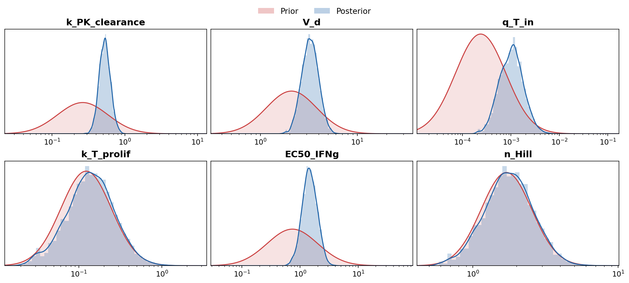
plot_marginals on fabricated samples. Parameters whose posterior is visibly tighter than the prior are well-constrained by the literature; ones still pinned to the prior bubble up the extraction-priority list.Stage 2: clinical data to final posterior
CalibrationTargets
Stage 2 inputs are CalibrationTargets, MAPLE’s sibling schema for clinical observables that require the full QSP simulator. A target wraps an observable (e.g. baseline immune cell densities in the tumor, or tumor volume at baseline + 6 weeks), the experimental scenario (dosing, biopsies, resections, intervention timing), and the Monte Carlo code that turns simulator output into the test statistic compared against the data.
Running the simulator
A simulate_with_parameters wrapper in qsp-hpc-tools runs the full QSP sims at the proposed parameters, with theta-hashed pool caching so repeated runs at the same draws hit the cache instead of re-simulating. The same wrapper backs both the inference-time training pool and posterior predictive checks at the end.
Pre-filtering implausible draws
A RestrictionClassifier (sklearn boosted trees on log-$\theta$) is fit on a pilot pool of $(\theta, \text{valid})$ pairs and rejects low-$P(\text{valid})$ draws before they hit the simulator. Most invalid draws are tumors that fail the evolve_to_diagnosis check (the simulated tumor never reaches detectable size in the given time window), so the classifier mostly filters out biologically implausible parameter combinations rather than solver crashes.
Neural posterior estimation
The Stage 1 posterior loads as a torch.distributions object and serves as the prior. The full-simulator likelihood $p(x_{\text{obs}} \mid \theta)$ has no closed form, so Stage 2 uses neural posterior estimation (NPE) via sbi: simulate many $(\theta, x)$ pairs from the prior, train a normalizing-flow conditional density estimator $q_\phi(\theta \mid x)$ on the pairs, and condition on the observed $x_{\text{obs}}$ to get $q_\phi(\theta \mid x_{\text{obs}})$ as the Stage 2 posterior.
Posterior predictive trajectories
For trajectory-level PPC (tumor volume curves over time, biomarker time courses, and so on), qsp_inference.inference.evaluate_calibration_target_over_trajectory evaluates a CalibrationTarget’s observable code over the long-form trajectory frames produced by qsp-hpc-tools’ assemble_evolve_trajectory_long. Trajectory plots therefore reuse the same observable definition the inference was conditioned on, rather than a re-implementation.
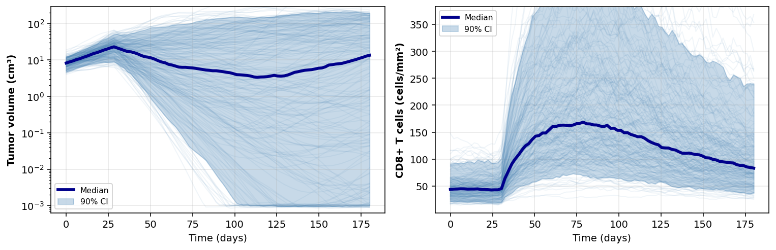
plot_posterior_predictive_spaghetti. Thin lines are individual posterior draws; the dark line is the median, the band is the 90% credible interval. Treatment kicks in at day 30.Diagnostics
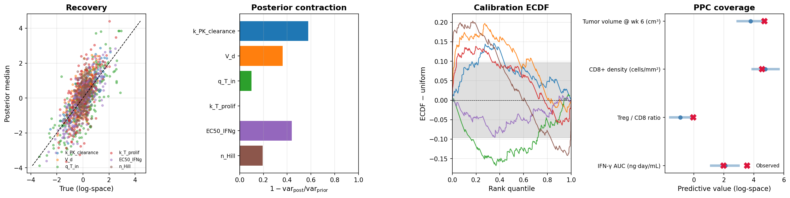
- Did the data tighten the parameter estimates? Posterior contraction $1 - \text{var}_{\text{post}}/\text{var}_{\text{prior}}$ per parameter, evaluated on a held-out test set of $(\theta, x)$ pairs from the simulator.
- Can the trained NPE recover the right parameters? Compare posterior medians against the held-out true $\theta$ (recovery $R^2$ per parameter).
- Are the credible intervals trustworthy? If they mean what they claim, the rank of each held-out true $\theta$ inside its posterior should be uniformly distributed (calibration ECDF).
- Can the calibrated model reproduce the observed clinical data? Posterior predictive coverage in the 90% PPC band per endpoint.
- Is the observed data weird relative to what the model predicts? Mahalanobis-$D^2$ of $x_{\text{obs}}$ against prior- and posterior-predictive samples, with a self-reference null so no chi-square assumption is needed.
- Which observables is the model fitting poorly? Drop each observable in turn and see how the joint Mahalanobis distance to the rest of the data changes (LOO predictive influence).
Audit (Stage 2 side)
The audit reads Stage 2 outputs back in and adds two report sections. The first covers per-parameter posterior shifts from the Stage 1 prior to the Stage 2 posterior, and re-runs the calibration check restricted to simulations whose observables are near the real data (since global calibration can look fine while calibration in the operating region is off). The second is clinical predictive uncertainty: a 95% CI per (scenario, endpoint) with attribution to PRCC-significant parameters, which feeds optimal Bayesian experimental design (OBED) for picking the next observable to constrain.
Stack
- MAPLE: schema-validated literature extraction into submodel targets
- qsp-codegen: SBML to C++ CVODE simulator
- qsp-hpc-tools: HPC orchestration and posterior-predictive sims
- qsp-inference: this package
Links
- GitHub repository
- Submodel inference guide
- Stage 2 SBI guide
- Stage 2 example script
- Stage 1 fast-iteration script
- Slide deck on Stage 1
References
- Tejero-Cantero, A., Boelts, J., Deistler, M., Lueckmann, J.-M., Durkan, C., Gonçalves, P. J., Greenberg, D. S., & Macke, J. H. (2020). sbi: A toolkit for simulation-based inference. Journal of Open Source Software, 5(52), 2505. Project site: sbi-dev.github.io/sbi.